🔧 Project

Single-Supply Half-Bridge Strain-Gauge Circuit

A full mixed-signal investigation: modelling a strain gauge in LTspice (which has no such element), building it into single- and dual-complementary half-bridges, then designing a single-supply AD8220 instrumentation-amplifier front end — gain, reference and all — to scale a ±37.5 mV bridge signal into a clean 0.6–4.4 V range an ADC can read.

LTspiceInstrumentation AmpAD8220Mixed-SignalAnalog Front End

Bridge

Dual-comp. half-bridge

Amplifier

AD8220 in-amp

Gain

50.4 V/V (R_G = 1 kΩ)

Supply

5 V single-rail

Reference

2.5 V

Output span

0.607 – 4.389 V

The problem: a signal that starts as a few millivolts

A strain gauge turns mechanical deformation into a tiny change in resistance. Put it in a bridge and, for the strains in this lab, you get a differential signal of at most a few tens of millivolts — riding on a large common-mode voltage. The whole exercise is two halves: model the sensor faithfully in simulation, then design the electronic interface that scales that millivolt signal up into a clean, single-supply range an ADC can actually digitize. I did it in three experiments, each building on the last.

1 · Modelling a strain gauge that doesn't exist in SPICE

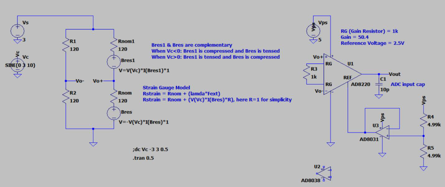
LTspice has no strain-gauge element, so the first task was to build one from the physics. A gauge's resistance follows

R_strain = R_nom + λ · F_ext

which I realised as a voltage-controlled resistor: a control voltage Vc stands in for the applied force, driving an arbitrary behavioural source V = V(Vc)·I(Bres)·R (with R = 1 for simplicity). That makes the voltage across the element equal to Vc at the branch current, i.e. a resistance you can sweep — so sweeping Vc from −3 to +3 sweeps the gauge through its full ±3 Ω of strain.

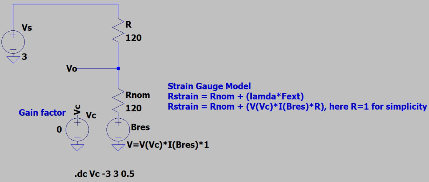
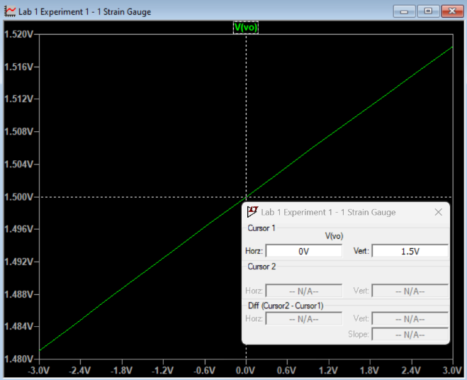
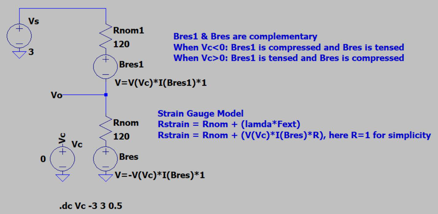
LTspice model of a single strain gauge as a voltage-controlled resistor in a voltage divider with a 120-ohm resistor. — Experiment 1 — a single 120 Ω gauge modelled as a controlled resistor, in a divider with a 120 Ω reference. Sweeping Vc emulates strain.

DC transfer curve of the single-gauge divider: output around 1.5 V, rising slightly with strain. — Its DC transfer curve — 1.5 V at zero strain, moving to 1.481 V / 1.519 V at the strain limits. Hand analysis and simulation matched to the millivolt.

With one gauge the useful swing is tiny (≈ ±18 mV about 1.5 V). Using a dual-complementary half-bridge — two gauges with opposite polarity, so one compresses as the other tenses — roughly doubles the signal and gives a clean, monotonic transfer characteristic (1.5 V at rest, 1.5375 V / 1.4625 V at the limits).

LTspice model of two complementary strain gauges forming a half-bridge. — The dual-complementary model — the second gauge's equation is negated so the two arms move in opposite directions, doubling the differential signal.

2 · The interface — an AD8220 instrumentation amplifier

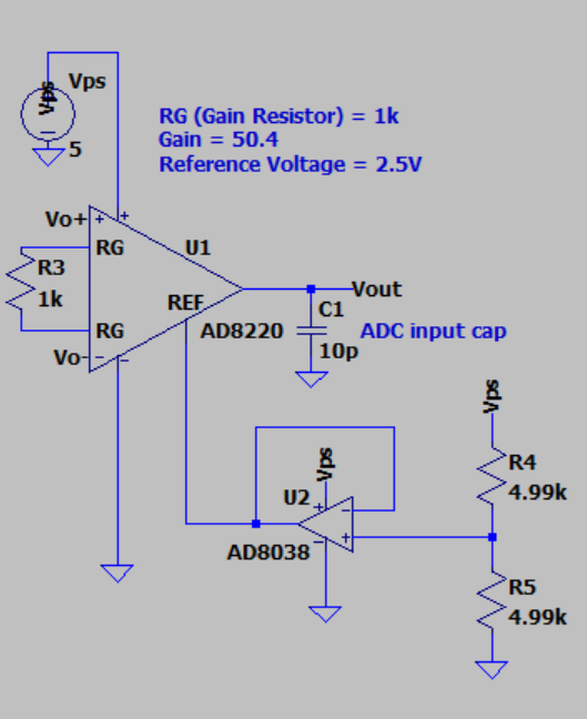
A few tens of millivolts sitting on a large common-mode voltage is exactly the job for an instrumentation amplifier. I built the half-bridge into an AD8220 in-amp on a single 5 V rail, with a 2.5 V reference to lift the bipolar bridge signal into the positive domain and a 10 pF cap standing in for the ADC's input.

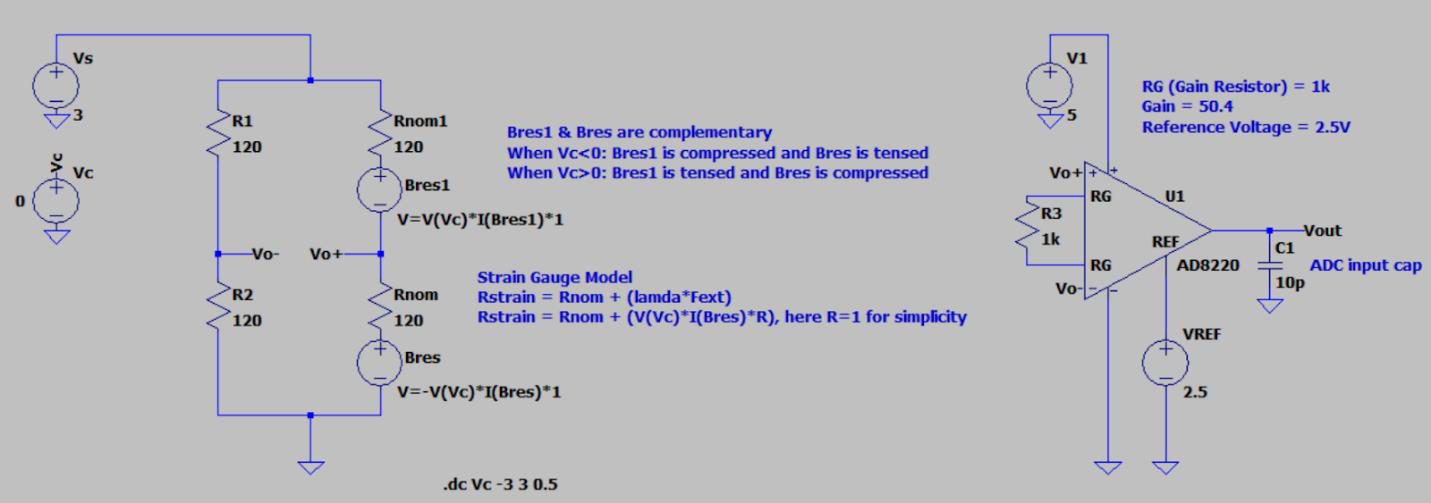
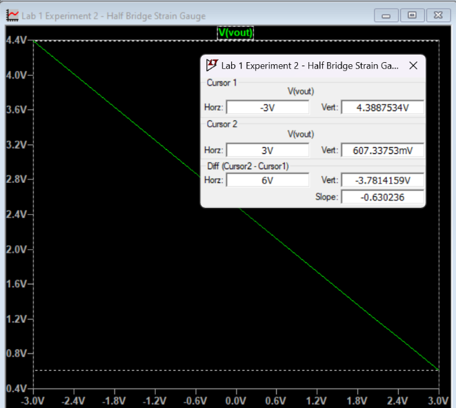
Complete Experiment 2 schematic: dual-complementary half-bridge feeding an AD8220 instrumentation amplifier with a 2.5 V reference. — The complete front end — dual-complementary half-bridge → AD8220 in-amp → ADC input, referenced to 2.5 V.

Choosing the gain was the real design decision. The half-bridge's maximum differential output was 37.5 mV. To use the amplifier's range without clipping, the output has to stay inside the AD8220's worst-case 4.7 V swing (over temperature), offset by the 2.5 V reference — which sets a ceiling of

(4.7 / 2) ÷ 0.0375 V ≈ 62.7 V/V

Picking a standard R_G = 1 kΩ gives G = 1 + 49.4 kΩ / R_G = 50.4 V/V — comfortably under the ceiling, so no useful signal is lost to clipping while still using most of the range. The result: 2.502 V at zero strain, swinging from 0.607 V to 4.389 V across full strain, matching hand calculation.

Amplified output transfer curve: V(vout) from 4.389 V at -3 V control to 0.607 V at +3 V control. — The amplified DC transfer characteristic — the ±37.5 mV bridge signal is now a full 0.607–4.389 V swing about the 2.5 V reference.

3 · Dynamic response

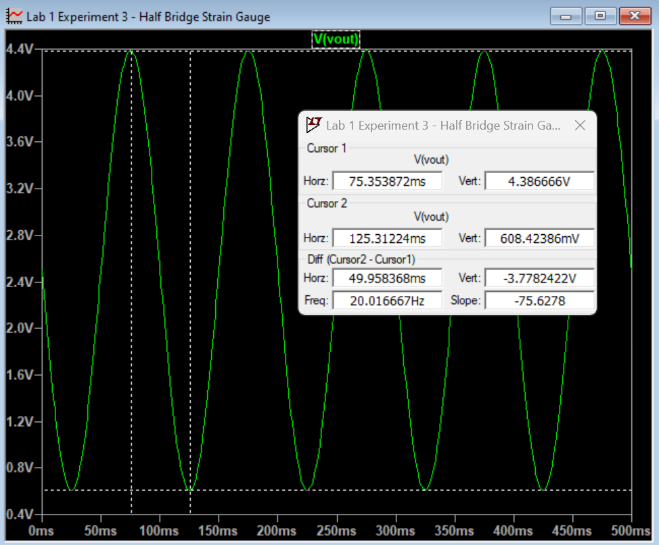
Static transfer curves only tell half the story, so I drove the strain with a 10 Hz sinusoid and ran a transient analysis. The amplified output tracks it cleanly between the same 0.607 V and 4.386 V limits — no clipping, no distortion of the meaningful swing, which confirms the gain and reference choices hold up for a real, time-varying strain.

Transient response: clean 10 Hz sinusoidal output swinging between about 0.61 V and 4.39 V. — Transient response to a 10 Hz sinusoidal strain — a clean, un-clipped swing between the min/max output levels.

4 · A real voltage reference, not an ideal one

An ideal 2.5 V source is fine in simulation but doesn't exist on a board, so the last step replaced it with the reference the AD8220 datasheet actually recommends: a resistor divider (two 4.99 kΩ) buffered by an AD8038 op-amp. I re-ran the 10 Hz test and the output was indistinguishable from the ideal-reference case — then swapped the buffer for an AD8031 and saw no change either, confirming the reference design is robust.

AD8220 instrumentation amplifier with an AD8038-buffered 4.99k/4.99k divider generating the 2.5 V reference. — The realistic front end — the 2.5 V reference now comes from a buffered divider (AD8038), exactly as the AD8220 datasheet prescribes.

Full Experiment 3 schematic with the buffered voltage reference and sinusoidal strain input. — The complete system with the practical reference and a sinusoidal strain stimulus.

What I took away from it

Building a behavioural device model from first principles when the simulator has no primitive for it — a voltage-controlled resistor standing in for a strain gauge.
Full analog-front-end design: bridge → instrumentation amp → reference → ADC input, sized end to end so a ±37.5 mV signal arrives clean and in range.
Gain selection as a headroom-vs-resolution trade — working back from the amplifier's swing and the reference to a concrete R_G.
Validating a design three ways — hand analysis, DC transfer, and dynamic transient — and moving from an ideal reference to the datasheet-recommended real one.
Why CMRR and high input impedance are the make-or-break specs for a bridge front end.